Local times and quadratic variation. Suppose we have a continuous local martingale (Mt)_{t >= 0}, where M_0=0. Let L_t^0 denote the local time of this process at zero.
Jadon Camacho
Answered question
2022-11-03
Suppose we have a continuous local martingale , where . Let denote the local time of this process at zero. I would like to prove the simple statement that:
where the bracket denotes the quadratic variation process.
My initial idea was to use the occupation density formula, which relates local times and the quadratic variation through the integrals involving non-negative Borel measurable functions. However, the formula integrates against the superscript of L rather than the subscript (that is, one measures the change with respect to the position of the process, not with respect to the time for a fixed position). Therefore, I do not hope that this could be useful.
I am not aware of any other (useful) results connecting the quadratic variation and the local times, so I would appreciate any help. I appreciate the fact that (heuristically) the local time measures the time a process spends at a particular point, with the clock given by the quadratic variation rather than the time indexing the process, but I can't quite get a rigorous proof of this.
Answer & Explanation
petyelebxu
Beginner2022-11-04Added 13 answers
By the theorem of Dubins and Schwartz, there is a Brownian motion B such that for all , a.s. The local times of B and M are related in the same way: . In particular, taking and defining , you have
Step 2
But as , you have as well, and so a.s. Therefore
Audrey Arnold
Beginner2022-11-05Added 2 answers
I'd just like to add an alternative solution, via the occupation and Tanaka formulas, which I found to be the most natural tools to use in the first place. We define:
to be the stopping times in question.
Step 2
1. To see that , we recall that by taking an appropriate modification of , we have via the occupation formula:
by continuity of M. Hence, the local time can start changing only after the quadratic variation.
2. To see that , by Tanaka's formula:
is a local martingale. By localizing, we get that for an appropriate sequence of stopping times increasing to infinity. Via Fatou's lemma and and continuity, this tells us that on , and so certainly , which means
New Questions in Algebra I
Find the volume V of the described solid S
A cap of a sphere with radius r and height h.
V=??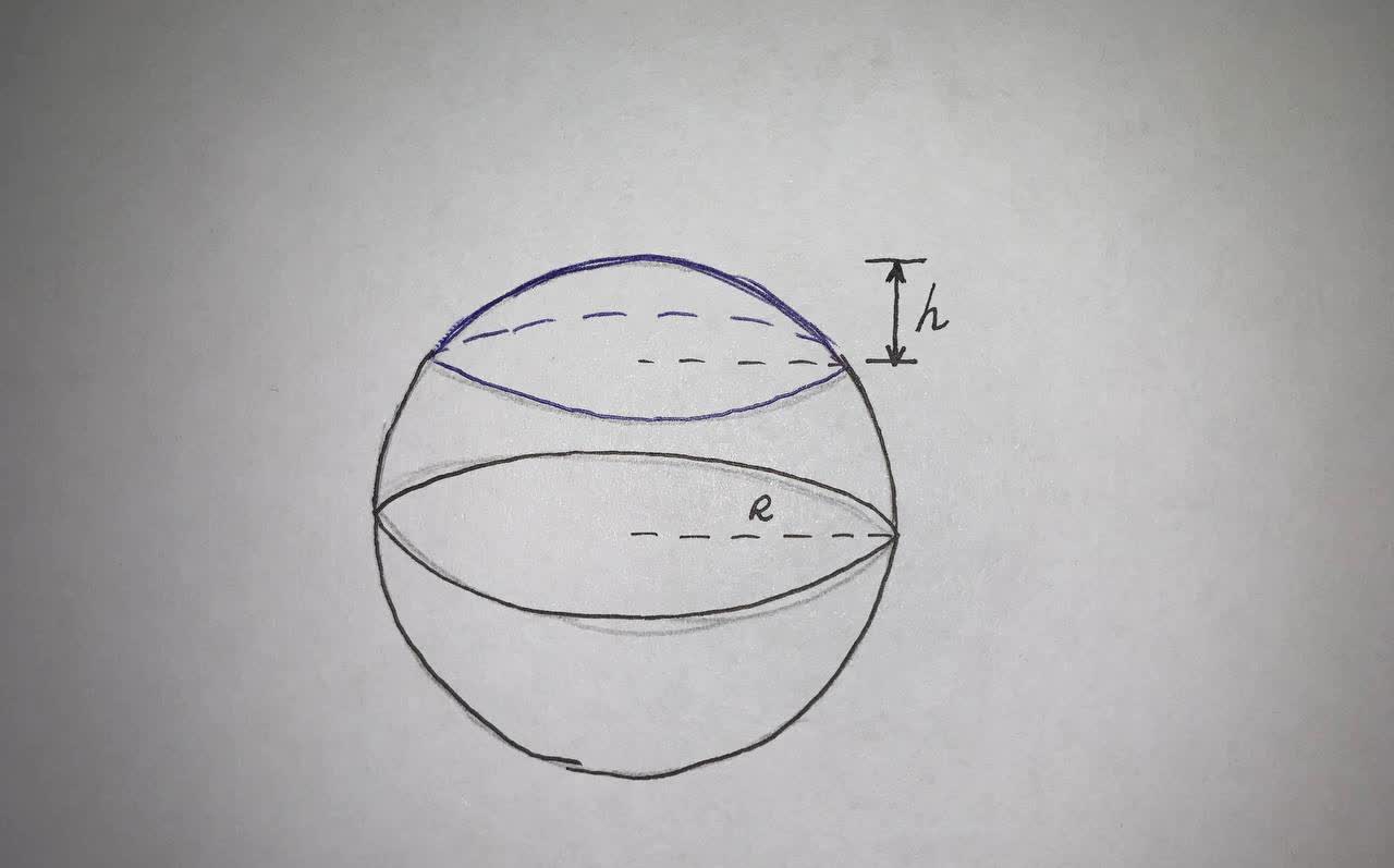
Whether each of these functions is a bijection from R to R.
a)
b)
c)
?In how many different orders can five runners finish a race if no ties are allowed???
State which of the following are linear functions?
a.
b.
c.
d.Three ounces of cinnamon costs $2.40. If there are 16 ounces in 1 pound, how much does cinnamon cost per pound?
A square is also a
A)Rhombus;
B)Parallelogram;
C)Kite;
D)none of theseWhat is the order of the numbers from least to greatest.
,
,
,
Write the numerical value of
Solve for y. 2y - 3 = 9
A)5;
B)4;
C)6;
D)3How to graph ?
How to graph using a table?
simplify
How to find the vertex of the parabola by completing the square ?
There are 60 minutes in an hour. How many minutes are there in a day (24 hours)?
Write 18 thousand in scientific notation.